You can just predict the optimum

instant Bayesian optimization! (kind of)

tl;dr: A 1-minute summary of this post

• The problem. Standard Bayesian optimization (BO) is powerful for finding optima (e.g., the best hyperparameters for a model), but the classic approach can be complex and inflexible. The loop of fitting a model and choosing where to sample next has many moving parts, and incorporating prior knowledge (an "educated guess") is surprisingly hard.
• The idea. Instead of this intricate loop, what if we could just predict the optimum directly? We propose reframing optimization as a large-scale prediction problem. We pre-train a transformer model (called ACE) on millions of synthetic optimization problems for which the solution is known in advance.
• How it works. For a new, unseen function, the model uses its "learned intuition" to directly predict a full probability distribution over the optimum's location and value from just a few initial samples. The key is a novel generative process we developed to create a massive dataset of complex functions with a guaranteed, known global optimum, which is what we need for training.
• Why it's neat. This "amortized" approach potentially makes optimization much faster at runtime. It simplifies the BO loop and makes it easy to incorporate user knowledge (priors) to guide the search more efficiently. This is a unifying paradigm that connects BO to other machine learning problems like simulation-based inference and image tasks.

Bayesian optimization (BO) is one of the pillars of modern machine learning and scientific discovery. It’s a standard tool for finding the best hyperparameters for a model, the ideal material composition, or the most effective drug compound. The textbook picture of BO is an elegant and simple loop: fit a probabilistic surrogate model (usually a Gaussian Process aka GP) to your observations, then optimize a so-called acquisition function to decide where to sample next, rinse and repeat.

While BO can be very fast nowadays and with solid implementations such as BoTorch, the classic loop can become intricate and sluggish once you move beyond the most basic or “vanilla” settings. There is a whole zoo of options to choose from: many different Gaussian Process kernels and an ever-growing list of acquisition functions (e.g., Expected Improvement, Upper Confidence Bound, Entropy Search, and many more). Moreover, something that seems like it should be simple in a method that has “Bayesian” in the name – for example, including an educated guess (a prior) about the location or value of the optimum – is not at all straightforward to incorporate into the standard GP framework.

But what if, instead of all this, we could just… predict the optimum?

The core idea I want to discuss in this blog post is this: if we are smart about it, we can reframe the entire task of optimization as a straightforward prediction problem.With the inevitable caveats, which we will cover later. Given a few samples from a function, we can train a neural network to directly output a probability distribution over the location $\mathbf{x}_{\text{opt}}$ and value $y_{\text{opt}}$ of the global optimum.In this post, we follow the convention that the goal is to *minimize* the function, so the global optimum is the *global minimum* of the function. This is one of the key applications of our recent work on the Amortized Conditioning Engine (ACE).

The core idea: learning from imagination

Think about how humans develop expertise. If you solve thousands of Sudoku puzzles, you don’t need to laboriously reason through every new puzzle from scratch. You start recognizing patterns. You get an intuition for where the numbers should go. You are, in a sense, predicting the solution based on the current configuration.More specifically, there are two distinct modules: a heuristic pattern-recognition module, which is what we are talking about now, and then there is a search/planning module, which we will get back to later.

We can do the same with machine learning. If we can generate a virtually infinite dataset of problems with known solutions, we can (pre)train a large model – like a transformer, the same architecture that powers modern Large Language Models (LLMs) – to learn the mapping from problem to solution. This is the essence of amortized inference or meta-learning. For a new problem, the model doesn’t need to reason from first principles; it makes a fast, amortized prediction using its learned “intuition”.These approaches are called "amortized" because the user pays a large upfront cost *once* for training the big network, but then obtains fast predictions at runtime (the small cost of a neural network forward pass). The large training cost is "amortized" over multiple later predictions, which are performed *without retraining*.

The main bottleneck for this approach is similar to the problem faced by modern LLMs: finding the training data. Where do we get a limitless dataset of functions with known optima?

While there are well-known techniques to generate functions (for example, using our old friends, the GPs), if we are required to optimize them to know their optimum, it looks like we are back to square one. The functions we want to train on are exactly those difficult, pesky functions where finding the optimum is hard in the first place. Generating such (function, optimum) pairs would be extremely expensive.

But it turns out you can do better than this, if you’re willing to get your hands dirty with a bit of generative modeling.

How to cook up a function with a known optimum

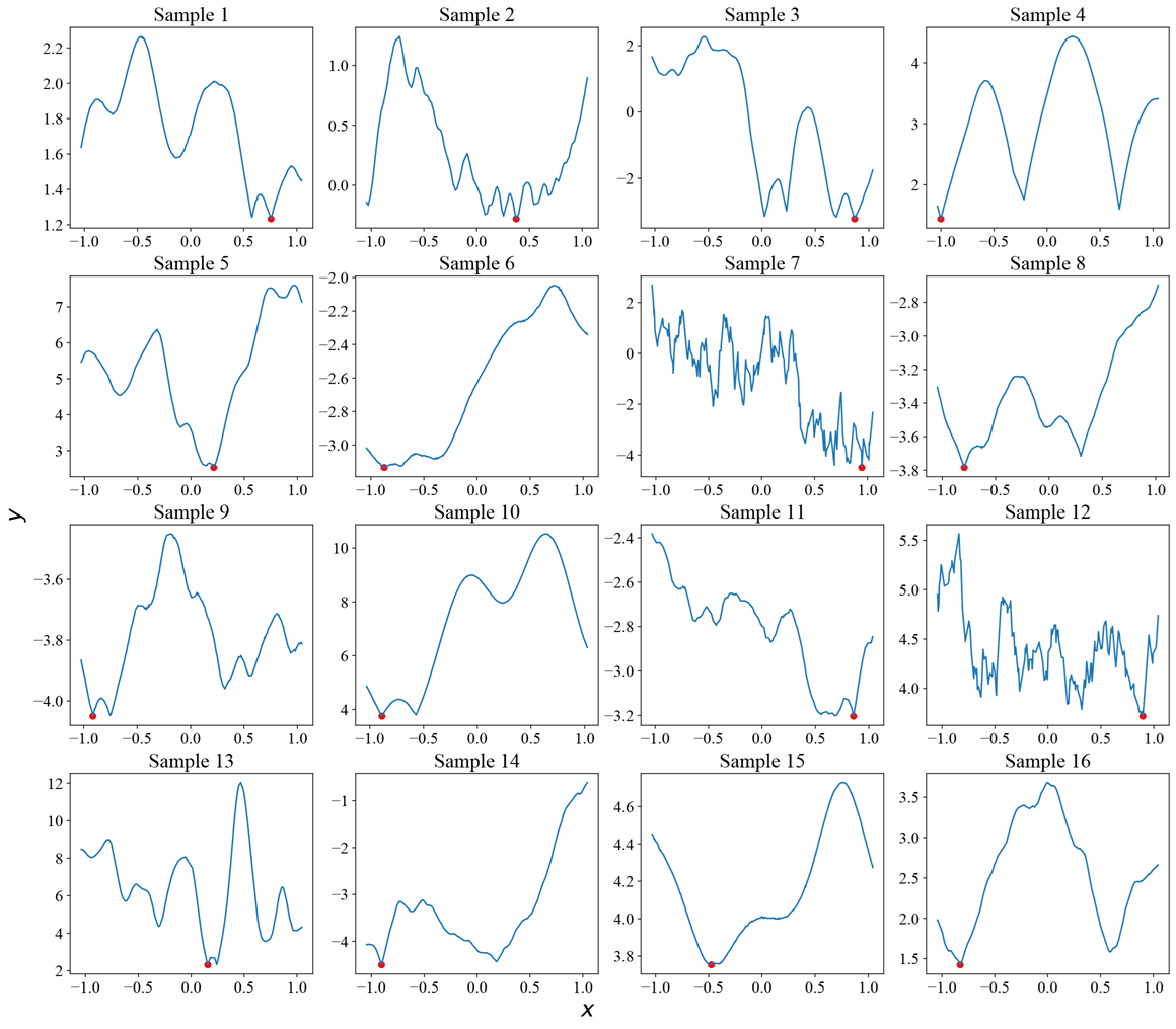
In our ACE paper, we needed to create a massive dataset of functions to train our model. The challenge was ensuring each function was unique, complex, and – most importantly – had a single, known global optimum $(\mathbf{x}_{\text{opt}}, y_{\text{opt}})$ which we could give our network as a target or label for training. Here is the recipe we came up with, which you can think of in four steps.

Step 1: Choose the function’s “character”

First, we decide what kind of function we want to generate. Is it very smooth and slowly varying? Is it highly oscillatory? We define this “character” by sampling a kernel for a Gaussian Process (GP), such as an RBF or Matérn kernel, along with its hyperparameters (like length scales). This gives us a prior over a certain “style” of functions.

Step 2: Pick a plausible optimum

Next, we choose a location for the global optimum, $\mathbf{x}_{\text{opt}}$, usually by sampling it uniformly within a box. Then comes an interesting trick. We don’t just pick any value $y_{\text{opt}}$. To make it realistic, we sample it from the minimum-value distribution for the specific GP family we chose in Step 1. This ensures that the optimum’s value is statistically plausible for that function style. With a small probability, we bump the minimum to be even lower, to make our method robust to “unexpectedly low” minima.

Step 3: Ensuring a known global optimum

Then, we generate a function from the GP prior (defined in Step 1) by conditioning it to pass through our chosen optimum location and value, $(\mathbf{x}_{\text{opt}}, y_{\text{opt}})$ established in Step 2. This is done by treating the optimum as a known data point.

However, simply forcing the function to go through this point is not enough. The GP is a flexible, random process; a sample from it might wiggle around and create an even lower minimum somewhere else by chance. To train our model, we need to be certain that $(\mathbf{x}_{\text{opt}}, y_{\text{opt}})$ is the true global optimum.

To guarantee this, we apply a transformation. As detailed in our paper’s appendix, we modify the function by adding a convex envelope. We transform all function values $y_i$ like this:

\[y_{i}^{\prime} = y_{\text{opt}} + |y_{i} - y_{\text{opt}}| + \frac{1}{5}\|\mathbf{x}_{\text{opt}} - \mathbf{x}_{i}\|^{2}.\]

Let’s break down what this does. The term $y_{\text{opt}} + |y_{i} - y_{\text{opt}}|$ is key. If a function value $y_i$ is already above our chosen optimum $y_{\text{opt}}$, it remains unchanged. However, if $y_i$ happens to be below the optimum, this term reflects it upwards, placing it above $y_{\text{opt}}$. This ensures that no point in the function has a value lower than our chosen minimum. Then, we add the quadratic “bowl” term that has its lowest point exactly at $\mathbf{x}_{\text{opt}}$.The $1/5$ is a magic number that governs the curvature of the bowl; you can change it. This bowl smoothly lifts every point of the function, but lifts points farther from $\mathbf{x}_{\text{opt}}$ more than those nearby. The result is a new function that is guaranteed to have its single global minimum right where we want it.The implementation in the paper is slightly different but mathematically equivalent: we first generate functions with an optimum at zero, apply a similar transformation, and then add a random vertical offset. The formula here expresses the same idea more directly.

This is a simple but effective way to ensure the ground truth for our generative process is, in fact, true. Without it, we would be feeding our network noisy labels, where the provided “optimum” isn’t always the real one.

Step 4: Final touches

With the function’s shape secured, we simply sample the data points (the (x, y) pairs) that we’ll use for training. We also add a random vertical offset to the whole function. This prevents the model from cheating by learning, for example, that optima are always near $y=0$.

By repeating this recipe millions of times, we can build a massive, diverse dataset of (function, optimum) pairs. The hard work is done. Now, we just need to learn from it.

Examples of one-dimensional functions with a known global optimum (red dot) from our training dataset. We can quickly generate a virtually infinite number of such functions in any dimension, with varying degrees of complexity.

A transformer that predicts optima

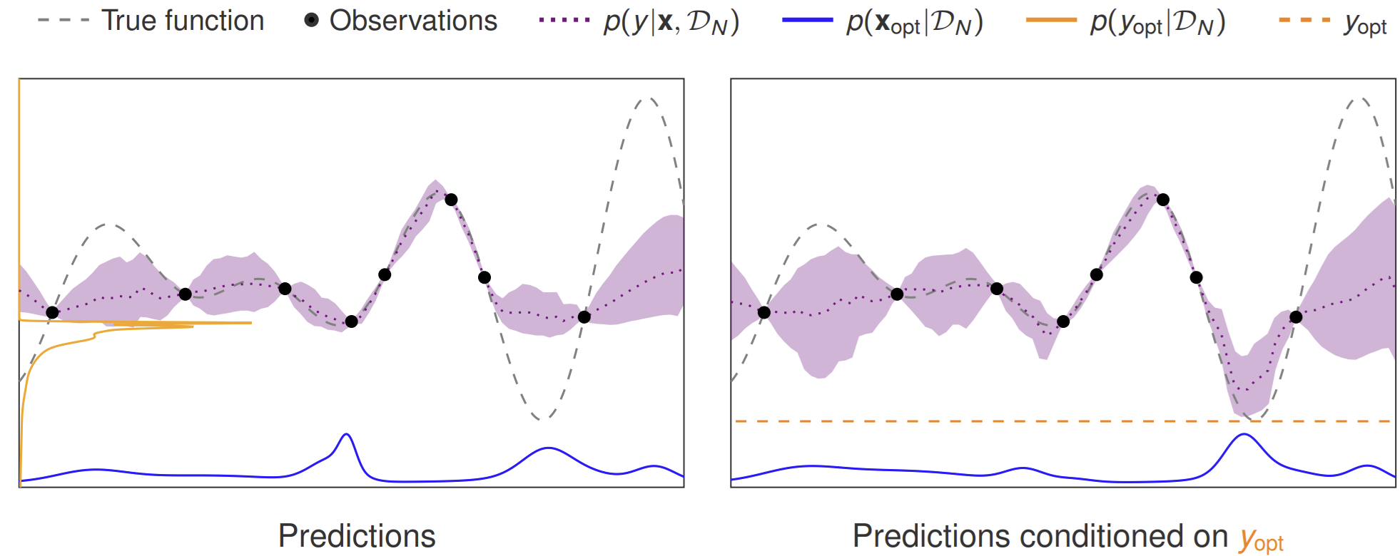
Once you have this dataset, the rest is fairly standard machine learning. We feed our model, ACE, a “context set” consisting of a few observed (x, y) pairs from a function. The model’s task is to predict the latent variables we care about: $\mathbf{x}_{\text{opt}}$ and $y_{\text{opt}}$. Here the term latent is taken from the language of probabilistic modeling, and simply means “unknown”, as opposed to the observed function values.

Because ACE is a transformer, it uses the attention mechanism to see the relationships between the context points and we set it up to output a full predictive distribution for the optimum, not just a single point estimate. This means we get uncertainty estimates for free, which is crucial for any Bayesian approach.

In addition to predicting the latent variables, ACE can also predict data, i.e., function values $y^\star$ at any target point $\mathbf{x}^\star$, following the recipe of similar models such as the Transformer Neural Process (TNP) and Prior-Fitted Networks (PFNs). ACE differs from these previous models in that it is the first architecture that allows the user to explicitly condition on and predict latent variables for the task of interest – such as the optimum location and value in BO –, and not just data points.

ACE can directly predict distributions over the optimum's location $p(x_{\text{opt}}|\mathcal{D})$ and value $p(y_{\text{opt}}|\mathcal{D})$ (left panel). These predictions can be further refined by conditioning on additional information, for example by providing a known value for the optimum $y_{\text{opt}}$ (right panel). Note that the predictions are sensible: for example, in the left panel, the prediction of the value of the optimum (orange distribution) is *equal or below* the lowest observed function value. This is not hard-coded, but entirely learnt by our network! Also note that the conditioning on a known $y_{\text{opt}}$ value in the right panel "pulls down" the function predictions.

The BO loop with ACE

So we have a model that, given a few observations, can predict a probability distribution over the optimum’s location and value. How do we use this to power the classic Bayesian optimization loop?

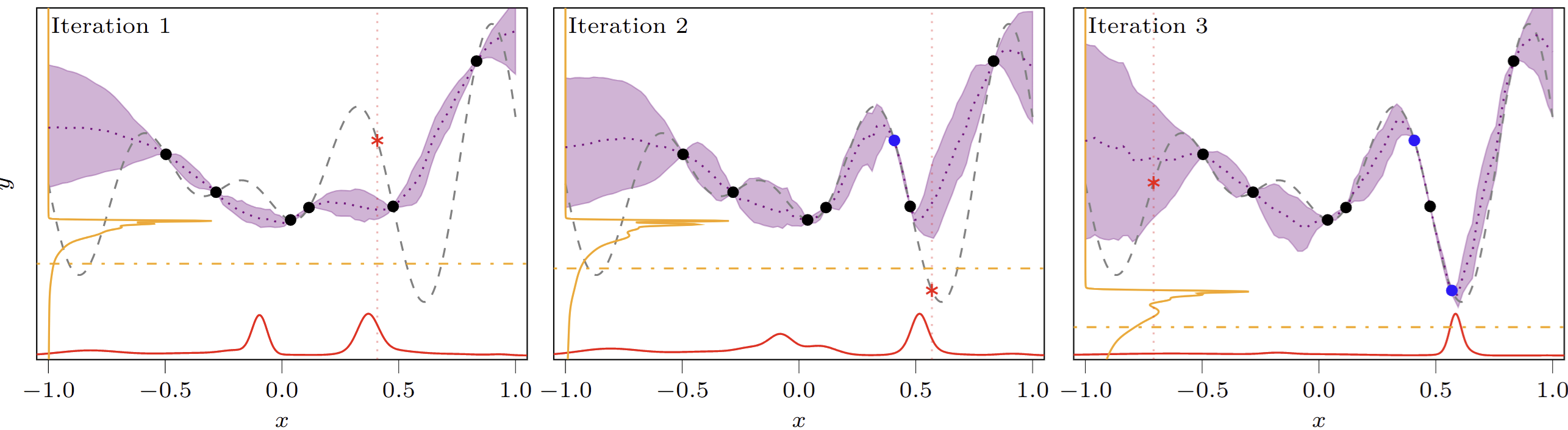
At each step, we need to decide which point $\mathbf{x}_{\text{next}}$ to evaluate. This choice is guided by an acquisition function. One of the most intuitive acquisition strategies is Thompson sampling, which suggests that we should sample our next point from our current belief about where the optimum is. For us, this would mean sampling from $p(\mathbf{x}_{\text{opt}}|\mathcal{D})$, which we can easily do with ACE.

But there’s a subtle trap here. If we just sample from our posterior over the optimum’s location, we risk getting stuck. The model’s posterior will naturally concentrate around the best point seen so far – which is a totally sensible belief to hold. However, sampling from it might lead us to repeatedly query points in the same “good” region without ever truly exploring for a great one. The goal is to find a better point, not just to confirm where we think the current optimum is.

This is where having predictive distributions over both the optimum’s location and value becomes relevant. With ACE, we can use an enhanced version of Thompson sampling that explicitly encourages exploration (see for a similar approach):

1. First, we “imagine” (aka phantasize) a better outcome. We sample a target value $y_{\text{opt}}^\star$ from our predictive distribution $p(y_{\text{opt}}|\mathcal{D})$, but with the crucial constraint that this value must be lower than the best value, $y_{\text{min}}$, observed so far.
2. Then, we ask the model: “Given that we’re aiming for this new, better score, where should we look?” We then sample the next location $\mathbf{x}_{\text{next}}$ from the conditional distribution $p(\mathbf{x}_{\text{opt}}|\mathcal{D}, y_{\text{opt}}^\star)$.

This two-step process elegantly balances exploitation (by conditioning on data) and exploration (by forcing the model to seek improvement). It’s a simple, probabilistic way to drive the search towards new and better regions of the space, as shown in the example below.

While this enhanced Thompson Sampling is powerful and simple, the story doesn’t end here. Since ACE gives us access to these explicit predictive distributions, implementing more sophisticated, information-theoretic acquisition functions (like Max-value Entropy Search or MES) becomes much more straightforward than in traditional GP-based BO, which requires complex approximations.

An example of ACE in action for Bayesian optimization. In each step (from left to right), ACE observes a new point (red asterisk) and updates its beliefs. The orange distribution on the left is the model's prediction for the optimum's *value* ($y_{\text{opt}}$). The red distribution at the bottom is the prediction for the optimum's *location* ($x_{\text{opt}}$), which gets more certain with each observation.

What if you already have a good guess?

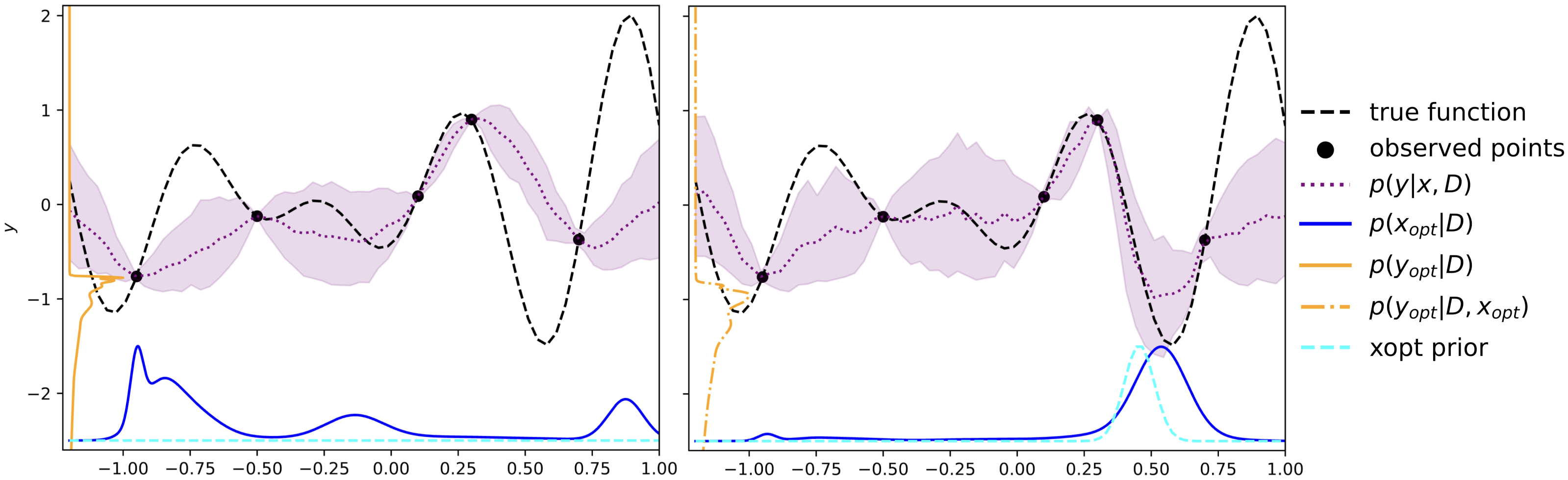
Predicting the optimum from a few data points is powerful, but what if you’re not starting from complete ignorance? Often, you have some domain knowledge. For example, if you are tuning the hyperparameters of a neural network, you might have a strong hunch that the optimal learning rate is more likely to be in the range $[0.0001, 0.01]$ than around $1.0$. This kind of information is called a prior in Bayesian terms.

Incorporating priors into the standard Bayesian optimization loop is surprisingly tricky. While the Bayesian framework is all about updating beliefs, shoehorning prior knowledge about the optimum’s location or value into a standard Gaussian Process model is not straightforward and either requires heuristics or complex, custom solutions (see, for example, ).

This is another area where an amortized approach shines. Because we control the training data generation, we can teach ACE not only to predict the optimum but also how to listen to and use a prior. During its training, we don’t just show ACE functions; we also provide it with various “hunches” (priors of different shapes and strengths) about where the optimum might be for those functions, or for its value. By seeing millions of examples, ACE learns to combine the information from the observed data points with the hint provided by the prior.

At runtime, the user can provide a prior distribution over the optimum’s location, $p(\mathbf{x}_{\text{opt}})$, or value $p(y_{\text{opt}})$, as a simple histogram across each dimension. ACE then seamlessly integrates this information to produce a more informed (and more constrained) prediction for the optimum. This allows for even faster convergence, as the model doesn’t waste time exploring regions that the user already knows are unpromising. Instead of being a complex add-on, incorporating prior knowledge becomes another natural part of the prediction process.

ACE can seamlessly incorporate user-provided priors. Left: Without a prior, the posterior over the optimum location is based only on the observed data. Right: An informative prior (light blue) about the optimum's location focuses the model's posterior belief (blue), demonstrating how domain knowledge can guide the optimization process more efficiently.

Conclusion: A unifying paradigm

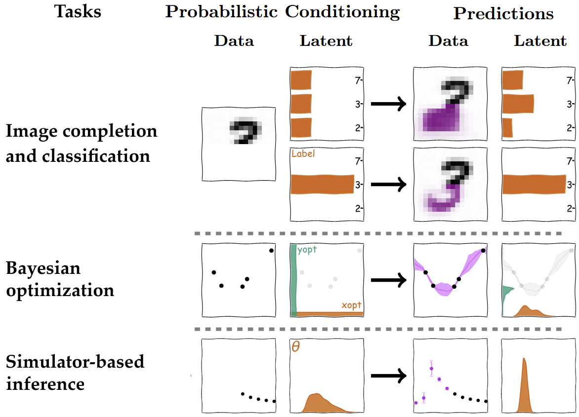
The main takeaway is that by being clever about data generation, we can transform traditionally complex inference and reasoning problems into large-scale prediction tasks. This approach unifies seemingly disparate fields. In the ACE paper, we show that the exact same architecture can be used for Bayesian optimization, simulation-based inference (predicting simulator parameters from data), and even image completion and classification (predicting class labels or missing pixels).

Everything – well, almost everything – boils down to conditioning on data and possibly task-relevant latents (or prior information), and predicting data or other task-relevant latent variables, where what the “latent variable” is depends on the task. For example, in BO, as we saw in this blog post, the latents of interest are the location $\mathbf{x}_{\text{opt}}$ and value $y_{\text{opt}}$ of the global optimum.

The ACE framework. Many tasks, like image completion and classification, Bayesian optimization, and simulation-based inference, can be framed as problems of probabilistic conditioning and prediction over data and latent variables.

This is not to say that traditional methods are obsolete. They provide the theoretical foundation and are indispensable when you can’t generate realistic training data. But as our simulators get better and our generative models more powerful, the paradigm of “just predicting” the answer is becoming an increasingly powerful and practical alternative – see for example this recent position paper, which makes similar points. Overall, it’s a simple idea, but it has the potential to change how we approach many hard problems in science and engineering.

Of course, there are some caveats...

The "just predict it" approach is powerful, but it's not magic -- yet. Here are a few limitations and active research directions to keep in mind:

• The need for known latents. The entire "learning from imagination" approach hinges on being able to generate a training dataset with known solutions (the latent variables). For Bayesian optimization, we showed a neat way to generate functions with a known optimum. But for other problems, generating this ground-truth data might be difficult, and you may have first to actually solve the problem for each training example.
• The curse of distribution shift. Like any ML model, ACE fails on data that looks nothing like what it was trained on. If you train it on smooth functions and then ask it to optimize something that looks like a wild, jagged mess, its predictions can become unreliable. This "out-of-distribution" problem is a major challenge in ML, and an active area of research.
• Scaling. Since ACE is based on a vanilla transformer, it has a well-known scaling problem: the computational cost grows quadratically with the number of data points you feed it. For a few dozen points, it's fast, but for thousands, it becomes sluggish. Luckily, there are tricks from the LLM literature that can be applied.
• From specialist to generalist. The current version of ACE is a specialist: you train it for one kind of task (like Bayesian optimization). A major next step is to build a true generalist that can learn to solve many different kinds of problems at once.

Teaser: From prediction only to active search

Direct prediction is only one part of the story. As we hinted at earlier, a key component of intelligence – both human and artificial – isn’t just pattern recognition, but also planning or search (the “thinking” part of modern LLMs and large reasoning models). This module actively decides what to do next to gain the most information. The acquisition strategies we covered are a form of planning which is not amortized. Conversely, we have been working on a more powerful and general framework that tightly integrates amortized inference with amortized active data acquisition. This new system is called Amortized Active Learning and Inference Engine (ALINE), where we use reinforcement learning to teach a model not only to predict, but also how to actively seek information in an amortized manner. But that’s a story for another day.

The Amortized Conditioning Engine (ACE) is a new, general-purpose framework for multiple kinds of prediction tasks. On the paper website you can find links to all relevant material including code, and we are actively working on extending the framework in manifold ways. If you are interested in this line of research, please get in touch!

Acknowledgments. This post was written with the assistance of Google's Gemini 2.5 Pro using Athanor, the open-source workbench for AI-assisted coding and writing.